

What if the 4.5% national jump in home prices actually tells a lie?
Across states, inventory was the main story.
Some states saw steep listing declines and 8–15% price gains. Others added lots of homes and saw flat or falling prices.
This post breaks down how state-level inventory swings move prices, why local factors like income and land limits matter, and what buyers, sellers, and investors should watch next: months of supply, new listings, and migration trends.
Short version: inventory mostly explains who wins and who doesn’t.
State-Level Overview of Inventory Shifts and Their Direct Impact on Home Prices
From Q4 2023 to Q4 2024, U.S. single-family home prices jumped 4.5% year over year according to the Federal Housing Finance Agency repeat-sales index, which tracks price changes on the same properties over time to avoid distortion from shifts in home type or quality. That national number hides serious state-by-state variation. Nearly every state’s price gain beat real GDP growth of 2.5% and inflation of 2.9% during the same stretch, but one state actually recorded a decline, and a few others saw double-digit appreciation. The difference? Inventory. States where active listings stayed far below pre-pandemic baselines (the entire Northeast cluster, for example) pushed prices higher. States where inventory surged (Mississippi saw listings climb while population stayed flat) watched prices flatten or drop. By July 2025, national housing inventory had climbed 26% year over year, the highest reading since at least 2017. But that inventory didn’t spread evenly, which kept pricing power in the hands of sellers in supply-starved markets and handed buyers fresh negotiating room in oversupplied metros.
A scatterplot linking state-level inventory change with price change usually shows an inverse relationship of around r ≈ −0.55. That means big inventory increases of 20 to 50% over twelve months often line up with price cooling of a few percentage points or outright drops, while inventory declines of 20% or more tend to match appreciation in the 8 to 15% range. But that’s not a universal law. States where income growth, in-migration, or tight land supply create structural limits can defy simple supply-and-demand logic. Connecticut, New Jersey, and Vermont all posted some of the nation’s strongest price gains in 2024 because their inventory stayed well below pre-pandemic norms, even as mortgage rates climbed above 7% at points during the year. Wyoming ranked among the top five fastest-appreciating states, driven by tourism demand near Yellowstone and other amenity zones, constrained housing supply, and steady in-migration pushing some properties into multi-million dollar range.
On the flip side, Mississippi was the only state with a year-over-year price decline from 2023 to 2024. Rising inventory met a buyer pool that didn’t grow. When listings climb and demand doesn’t, prices give. Housing Market Snapshot: Price Changes by State breaks down annual state-level price movements and shows just how few markets dodged upward pressure entirely. The five clearest patterns from the inventory-price data:
- Inventory declines of 20% or more usually drive annual price gains of 8 to 15%, especially in states with months of supply below 2.5 and solid income growth.
- Inventory increases of 15% or more often slow price appreciation to 0 to 3% or produce outright declines of 1 to 5%, particularly where population and job growth stall.
- States with months of supply below 2.5 see rapid price acceleration, as even small demand bumps exhaust available listings within weeks.
- States where months of supply tops 4.0 shift negotiating power to buyers, lengthening marketing times and increasing price cuts and below-list offers.
- Structural supply limits (coastal geography, restrictive zoning, scarce buildable land) amplify the price response to any inventory change, making 10% swings in listings produce 4 to 8% price moves within six to twelve months in supply-constrained markets.
Regional Inventory Patterns Influencing Home Prices Across the U.S.

The Northeast entered 2024 with inventory far below pre-pandemic norms, and it stayed that way. Active listings in Connecticut, New Jersey, Vermont, and nearby states remained tight throughout the year, supporting some of the nation’s strongest price appreciation. Higher median incomes helped buyers absorb elevated mortgage costs, and limited buildable land in many suburban corridors kept new construction from flooding the market. Sellers in the Northeast kept pricing power even as mortgage rates hovered in the mid-6% to low-7% range. Days on market stayed short, multiple-offer scenarios remained common in desirable school districts and commuter towns, and price cuts were rare. The Northeast’s inventory scarcity acted as a floor under prices. Any small uptick in demand translated directly into bidding pressure.
The South, particularly large Sun Belt metros, saw the opposite. States that built extensively during the pandemic (Florida, Texas, Georgia, North Carolina, Nevada) now carry bigger inventory backlogs as demand softened in 2024. Raleigh saw inventory jump 54.5% year over year by July 2025. Las Vegas rose 43.1%, Miami climbed 40.1%, Atlanta added 36.7%, and Houston recorded a 30.9% increase. Those inventory surges didn’t trigger immediate price collapses, but they did slow appreciation and shift leverage toward buyers. Parts of coastal Florida and Texas are expected to cool further as insurance costs climb, job growth moderates, and investor interest fades. Rising supply meeting weakening demand fundamentals creates conditions for flat or slightly negative price movement in select Sun Belt markets over the next twelve months.
The Midwest and Great Lakes region sits somewhere between those two extremes. Inventory increases have been modest compared to the Sun Belt. Chicago posted the smallest year-over-year gain among major metros at just 6.7%, and affordability remains relatively strong. Analysts expect these areas to heat up as buyers priced out of coastal and high-growth Southern markets look for lower entry prices and stable job markets. Columbus saw inventory rise 29.9%, and Louisville climbed 36.5%, but both cities maintain job growth and population inflows that should prevent the kind of demand collapse seen in overbuilt Sun Belt suburbs. The Midwest’s housing stock per capita is larger than many coastal states, which usually cushions price swings. But pockets near major employers or universities can tighten quickly when local demand picks up.
The West shows the widest internal variation. California metros like San Diego reported inventory increases of 32.4% year over year, yet median prices in the state remain elevated because coastal land constraints, strict zoning, and high incomes keep structural demand strong. Denver’s inventory rose 30.1%, but in-migration from the coasts and a diverse economy have prevented a full demand retreat. Parts of the Mountain West with smaller populations and tourism-dependent economies (Wyoming being a notable outlier due to its scarcity and high-end migration) can see large percentage swings in inventory that matter less in absolute terms. A few dozen extra listings in a small county can skew year-over-year comparisons without fundamentally altering the market. Across the West, the interplay of geography, income, and migration determines whether rising inventory translates into buyer opportunity or simply a return to pre-pandemic norms.
Inventory Metrics That Drive Price Movement by State

Active listings count the number of homes currently available for purchase in a given state or metro, the raw supply at any moment. Months of supply divides active listings by the monthly sales pace, translating inventory into a time estimate: how long it would take to sell every listed home if no new listings appeared. New listings measure fresh supply hitting the market each month, while pending sales (homes under contract but not yet closed) signal near-term demand and future closed volume. Days on market tracks how long the typical home sits before going under contract, a speed indicator that reflects competition. Median sale price captures the middle value of all closed transactions in a period, less sensitive to outliers than mean price but still responsive to mix shifts when higher or lower-priced homes dominate monthly sales.
States with months of supply below 2.5 usually see rapid price appreciation because buyers outnumber available homes, creating bidding pressure and above-list offers. A 10% drop in inventory in such a market can push prices 4 to 8% higher within six to twelve months, especially where local income growth supports affordability. States with months of supply above 4.0 hand leverage to buyers: homes linger, sellers cut prices to attract offers, and negotiation becomes normal rather than the exception. Days on market stretch from under two weeks to over a month, and the odds of selling above list price fall sharply. Tracking these metrics month over month reveals inflection points. When inventory crosses the 3-month threshold upward, pricing power begins to shift. When it falls below 2 months, seller advantage intensifies.
Twelve-month correlations between inventory change and price change provide a numerical snapshot of the relationship’s strength in each state. A correlation coefficient of r ≈ −0.55 is typical at the national level, indicating a moderate inverse link: as inventory rises, price growth tends to slow, and vice versa. But state-by-state results vary widely. Supply-constrained coastal markets often show stronger correlations (r ≈ −0.68 or lower) because any supply movement has outsized effects. States with elastic supply (flat land, relaxed zoning, active homebuilders) show weaker correlations because new construction can absorb demand shocks without large price swings. Inventory declines of 20% or more frequently align with annual price gains of 8 to 15%, while inventory increases of 20 to 50% can slow growth to low single digits or trigger 1 to 5% declines. Buyers, sellers, and investors who monitor these six metrics gain early warning of market shifts:
- Active listings (absolute count and year-over-year % change) to gauge total supply and direction.
- Months of supply to understand whether the market favors buyers (above 4), sellers (below 2.5), or sits balanced (2.5 to 4).
- New listings per month to spot supply acceleration or deceleration before it shows up in active inventory.
- Pending sales count to measure near-term demand and predict closed-sale volume one to two months ahead.
- Days on market (median or average) to assess competitive intensity and pricing discipline.
- Median sale price and year-over-year % change to track the outcome of supply-demand dynamics in dollar terms.
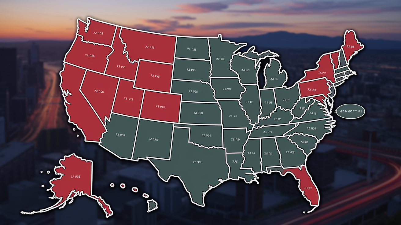
Geographic Visualization of Inventory and Price Shifts by State

Maps turn raw inventory and price numbers into patterns anyone can read at a glance. A U.S. choropleth (color-coded) map showing each state’s year-over-year inventory change from Q4 2023 to Q4 2024 reveals regional clusters: deep reds in the Northeast where listings fell or stayed flat, warm oranges and yellows across parts of the Midwest, and greens or blues blanketing Sun Belt states where inventory surged. Overlay a second map of price-change percentages for the same period, and the inverse relationship jumps out. States colored dark red for inventory drops often wear dark green for price gains, while states flooded with new listings show cooler price performance. Side-by-side maps make it easy to spot outliers and test assumptions.
A scatterplot plots each state as a single dot, with inventory change on the x-axis and price change on the y-axis. A downward-sloping regression line through those dots shows the typical inverse correlation (r ≈ −0.55 nationally), and states that sit far from the line reveal unique local dynamics. Strong job growth, insurance shocks, or migration anomalies that break the usual pattern. Labeling each dot with the state abbreviation lets readers find their own market instantly. Adding a third dimension (bubble size for population or median income) can highlight which large or wealthy states defy gravity.
Ranked tables complement maps and scatterplots by offering precise numbers. A table listing all 50 states with columns for active listings, year-over-year inventory change (%), months of supply, median sale price, and year-over-year price change (%) gives analysts and consumers the raw data to run their own comparisons. Sorting by inventory change ascending or descending surfaces the extremes: which states tightened most (lowest inventory growth or largest declines) and which flooded (highest inventory increases). Regional time-series panels, line charts tracking inventory and median price month-by-month for the Northeast, South, Midwest, and West over a three to five-year window, show whether recent shifts are cyclical blips or structural trends.
- Choropleth map of % inventory change by state (July 2025 or latest quarter) to show geographic clustering and regional divergence at a glance.
- Scatterplot with state labels, inventory % change (x-axis) vs. price % change (y-axis), regression line, and displayed correlation coefficient to reveal the strength and exceptions to the inverse relationship.
- Ranked state table with columns for active listings, % inventory change, months of supply, median sale price, and % price change to provide sortable, precise data for every market.
- Regional time-series line charts (2017 to 2025) tracking inventory and median price for the four major U.S. regions to distinguish short-term shocks from long-run trends.
Case Studies: How Inventory Changes Impact Prices in Specific States

Northeast Example (CT/NJ/VT): Low Inventory, High Appreciation
Connecticut, New Jersey, and Vermont formed the core of the “Northeast cluster” that posted the nation’s strongest price gains from Q4 2023 to Q4 2024. All three states entered the period with active listings far below pre-pandemic levels, a legacy of limited new construction, restrictive zoning in many towns, and geographic constraints (coastline, mountains, existing dense development). When mortgage rates climbed above 6.5% in early 2024, many potential sellers chose to stay put rather than give up sub-4% loans, tightening supply further. At the same time, high median household incomes in suburban corridors around New York City and in Vermont’s amenity towns kept qualified buyer pools larger than inventory could satisfy. The result was sustained bidding pressure, short days on market, and price appreciation that outpaced national averages by several percentage points. Even modest upticks in demand, a new employer, a strong stock-market quarter boosting bonuses, translated directly into higher sale prices because there were so few homes to compete for.
Mississippi: Inventory Increase and Price Decline
Mississippi was the only U.S. state to record a year-over-year home-price decline from 2023 to 2024. The cause was straightforward: inventory rose while population remained flat. Without new households moving in or forming, the buyer pool didn’t grow, but the number of homes listed for sale did. That imbalance handed leverage to the shrinking set of active buyers, who could negotiate price cuts, request repairs, and walk away if terms didn’t suit them. Sellers who needed to move faced longer marketing times and had to adjust list prices downward to attract offers. The state’s relatively low median income also meant fewer buyers could qualify at prevailing mortgage rates, compressing the upper end of the market. Mississippi’s case shows the textbook outcome when inventory expands into stagnant or declining demand: prices give way.
Wyoming: In-Migration, Scarcity, and High-End Demand
Wyoming ranked among the top five states for price appreciation despite being outside the Northeast, driven by constrained housing supply and sustained in-migration from higher-cost states. Tourism and amenity demand, particularly in areas near Yellowstone National Park and Jackson Hole, pushed property values into multi-million dollar territory for certain segments. The state’s small population means even a few hundred new high-income households moving in can tighten inventory significantly. Buildable land is limited by federal ownership, topography, and infrastructure constraints, so new construction struggles to keep pace with demand spikes. Existing homes in desirable locations command premium prices, and sellers enjoy negotiating leverage similar to coastal markets. Wyoming’s experience shows that low absolute inventory in a small state can produce large percentage price gains when migration and income trends align.
Sun Belt States: Pandemic-Era Building and Cooling Prices
Large Sun Belt metros that built aggressively during the pandemic now carry inventory surpluses that have begun to cool price growth. Raleigh’s inventory surged 54.5% year over year by July 2025, Las Vegas climbed 43.1%, and Miami rose 40.1%. All three reflect completed construction projects hitting the market and softening buyer demand as mortgage rates stayed elevated and some pandemic-driven migration reversed. While none of these markets experienced the kind of price collapse seen in past cycles, appreciation slowed to low single digits or flattened entirely in certain submarkets. Investors who bought rental properties in 2021 to 2022 faced thinner cash flows as rent growth decelerated and vacancy rates ticked up. Parts of Texas and coastal Florida are expected to cool further over the next year as insurance costs rise, job growth moderates, and the pipeline of newly built homes continues to close. The Sun Belt’s experience demonstrates that even strong fundamentals can’t prevent near-term price moderation when inventory surges outpace demand.
Short-Term vs Long-Term Inventory Shocks and Their State-Level Price Effects

Short-term inventory shocks, sudden jumps or drops in active listings over a few months, can distort pricing signals without changing the underlying market structure. A wave of delayed spring listings hitting in May and June might spike inventory 15% month over month, but if buyer activity picks up at the same time due to school-year timing, prices may barely budge. A harsh winter or natural disaster can pull inventory off the market temporarily, creating artificial scarcity that lifts prices until supply normalizes. These cyclical swings matter for timing individual transactions but rarely alter a state’s multi-year price trajectory. Pandemic-era construction in certain Sun Belt states created a medium-term supply pulse. Projects started in 2021 finished in 2023 and 2024, flooding local markets with new inventory just as demand cooled. That overhang can suppress prices for one to three years until absorption catches up.
Structural shortages exert persistent upward pressure on prices regardless of short-term inventory movements. Researchers estimate the U.S. needs roughly 3 to 4 million additional homes beyond normal annual construction to remedy the deficit accumulated since the 2008 housing crash and subsequent decade of underbuilding. States with the largest shortfalls (often high-cost coastal markets and fast-growing Sun Belt metros) will see prices remain elevated even when monthly inventory ticks up, because the gap between households and housing units hasn’t closed. In these markets, a 20% year-over-year inventory increase might bring listings from “severely constrained” to “tight” rather than “balanced,” leaving sellers with leverage and prices rising, just at a slower pace. Structural shortages also make any easing of zoning or acceleration of permits highly price-relevant. Adding even a few hundred units per quarter in a supply-starved metro can moderate price growth noticeably.
| Type of Inventory Change | Typical Drivers | Expected Price Effect |
|---|---|---|
| Short-Term Shock | Seasonal listing patterns, weather events, temporary demand drop (e.g., rate spike), delayed construction completions | Price volatility over 1 to 6 months; usually mean-reverts once the shock fades; can create brief buyer or seller windows but rarely alters long-run trend |
| Structural Shortage | Decade of underbuilding post-2008, restrictive zoning, geographic constraints, slow permit approvals, high construction costs | Sustained upward price pressure over years; even rising inventory may not bring prices down if deficit remains large; easing only occurs with multi-year construction ramp or demand collapse |
| Pandemic-Era Oversupply | Rapid construction 2020 to 2022 in select Sun Belt metros, speculative investor buying, then demand softening as migration slows and rates rise | Price moderation or decline over 1 to 3 years in affected metros; absorption eventually clears excess; risk of localized price drops if job growth stalls or insurance/tax costs spike |
Policy and Zoning Forces Shaping Inventory and Price Outcomes by State

Coastal and densely developed urban markets operate under strict land-use regulations that limit supply elasticity. When demand rises, builders can’t simply clear new land and put up subdivisions. Instead, they navigate lengthy permitting processes, height restrictions, environmental reviews, and neighborhood opposition. Even modest increases in buyer interest push prices sharply higher because new supply can’t respond quickly. States like California, New York, and Massachusetts show this pattern: a 10% inventory decline can drive prices up 6 to 10% within a year, while a 10% inventory increase barely dents appreciation because the structural shortage remains. Zoning reform, allowing accessory dwelling units, reducing minimum lot sizes, or permitting multi-family construction in single-family zones, can incrementally boost inventory. But the effects take years to compound and require sustained political will.
States with more permissive land-use policies and abundant flat, buildable land (parts of Texas, the Carolinas, Georgia, Arizona) show weaker price responses to short-term inventory changes because builders can ramp production when prices rise. That supply elasticity acts as a brake on price acceleration, which benefits affordability but also means sellers capture less appreciation during booms. Permitting rates offer a forward-looking signal: states where single-family permits grew 15% or more annually over the past few years are likely to see larger inventory increases and slower price growth in the near term, while states where permits have stagnated or declined face ongoing supply constraints that support higher prices. Policy interventions to increase supply, streamlined permitting, tax incentives for construction, public land releases, take time to flow through to active listings. But when they do, they can shift a state from structurally tight to balanced, altering the price outlook for years.
Buyer, Seller, and Investor Strategies Based on State Inventory Conditions

Buyers in low-inventory states should move quickly once they identify a target property. Pre-approval matters more than ever. Sellers and listing agents prioritize offers from buyers with verified financing and minimal contingencies. Expect competition: multiple offers, escalation clauses, and above-list sale prices remain common in markets where months of supply sits below 2.5. Stretching budget to win a bidding war is tempting, but rising mortgage rates mean monthly payments can jump faster than home values, so stress-test affordability at rates 0.5 to 1.0 percentage points higher than today’s quote. In high-inventory states, buyers gain negotiating leverage. Request repairs, ask for closing-cost credits, and don’t hesitate to walk if inspection reveals issues. Another property will likely appear soon. Timing listings and price cuts in these markets can surface deals. Homes that have sat for 45 to 60 days often see sellers willing to negotiate.
- Secure mortgage pre-approval with a local lender before touring homes to demonstrate readiness and avoid losing out to faster-moving buyers in tight markets.
- Monitor days-on-market trends weekly in your target metro; if the median rises above 30 days, shift from urgency to patience and use that time to negotiate.
- In low-inventory states, prioritize properties priced at or slightly below comparable sales to avoid overpaying in a bidding war; let others chase the premium listings.
- Track new-listing volume and pending-sale counts to identify early signs of inventory loosening, which can create brief buyer windows before broader market awareness.
- In high-inventory metros, request seller concessions (repairs, rate buy-downs, closing costs) because longer marketing times make sellers more flexible.
Sellers in low-inventory markets can price aggressively, often at or above recent comparable sales, and still receive multiple offers within days. Staging, professional photos, and weekend open houses amplify competition and drive final prices higher. But rising mortgage rates present a risk: even in tight markets, affordability limits exist, so overpricing by more than 5 to 10% can cause a listing to stall. Once a home sits for three weeks, buyer interest cools quickly. In high-inventory states, pricing discipline is essential. Start at or slightly below market to generate early showing activity and create urgency, because properties that linger get mentally categorized as “stale” by buyers and agents. Investors targeting buy-and-hold should focus on states where inventory is tightening relative to pre-pandemic levels and where local income growth supports rent and resale appreciation. Avoid markets with growing inventory, flat or declining population, and deteriorating job fundamentals unless the strategy involves deep value-add renovation or short-term rental arbitrage in tourist zones.
- Price at or just below recent comparable sales if inventory is rising in your metro to generate showings in the first two weeks and avoid the “stale listing” penalty.
- In low-inventory markets, prepare for above-list offers by setting your initial ask conservatively, then let competition drive the final price rather than starting high and cutting later.
- Monitor local months of supply monthly; if it crosses above 3.5 months, adjust expectations and be ready to negotiate rather than hold firm on price.
- For investors, target states with 12-month inventory declines of 15% or more, positive net migration, and job growth above 1% annually to capture structural appreciation.
- Avoid markets where inventory has risen 20%+ year over year and population growth is flat or negative unless cash flow from rents can sustain the hold period through a price-correction cycle.
Final Words
Inventory shifts are the main dial for prices right now: low supply in the Northeast and places like Wyoming pushed gains, while big inventory jumps in parts of the Sun Belt and Mississippi cooled or reversed prices.
Watch months-of-supply, active listings, and short-term spikes — they predict local price moves better than national headlines.
Knowing how inventory changes impact home prices by state gives you a clear game plan: buyers, sellers, and investors can act with data, not guesswork. There’s opportunity if you follow the local signal.
FAQ
Q: What is the 3-3-3 rule in real estate?
A: The 3-3-3 rule in real estate is an informal agent heuristic that varies by market; commonly it signals a 3% pricing band, the first 3 days to gauge buyer interest, and a 3‑week window for offers.
Q: Which state has the most housing inventory?
A: The state with the most housing inventory changes monthly; recently Sun Belt states like Texas and Florida showed the largest inventory gains, so check current state-level listings or the VisualCapitalist map for the latest leader.
Q: What is the hardest month to sell a house?
A: The hardest month to sell a house is usually December, with January close behind, because holiday timing and winter weather cut buyer activity, causing longer days on market and weaker offers.
Q: What happens to home prices if the stock market crashes?
A: Home prices after a stock market crash typically cool or fall, but the size depends on job losses, credit tightening, and interest rates — housing often lags, so regional outcomes can be mixed.